Before going into how one can parallelize MOOSE, it is absolutely necessary that one has a good understanding of how MOOSE actually works... serially. Here, I will just outline the theory behind the sort of computations that are done in MOOSE. In a future post, I will go into the details of the actual code for the solver in MOOSE.
We saw the general equation of the neuron in the first post. Heres a refresher:
We saw the general equation of the neuron in the first post. Heres a refresher:
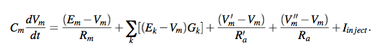
Don't hesitate to scroll down and check out that post if you don't remember this equation.
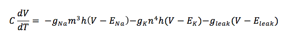
Let's simplify this equation a bit. We'll remove the resistance considerations and expand that summation to allow for only Sodium and Potassium ion channels, as these account for the vast majority of current changes in the cell. We will also assume that there are no injection currents for now. The new equation then becomes:
Let's simplify this equation a bit. We'll remove the resistance considerations and expand that summation to allow for only Sodium and Potassium ion channels, as these account for the vast majority of current changes in the cell. We will also assume that there are no injection currents for now. The new equation then becomes:
Now this equation, as you can see, is a time integral. So it assumes that voltages are constant over space. However, this is not true. Even within a single compartment, voltages can vary considerably from one end to the other. So, accuracy of models can be increased substantially by integrating over space along with time. This leads to conversion of the above equation - an Ordinary Differential Equation, into a Partial Differential Equation. Let's see what that looks like
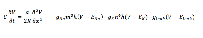
So this is an equation in which the voltage varies continuously with both space and time! That's a pretty hard equation to solve. A clever trick called the method of lines reduces this PDE into a set of 'coupled' ODEs, which basically means that the ODEs all depend on each other. Although this mutual dependence means that the ODEs can't be solved by straightforward differentiation, they are far easier to solve than PDEs. This gives us the equation below:
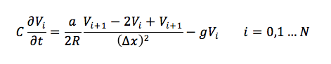
Note that we've also reduced all those gV terms into one for brevity.
This is an interesting equation. It removes the dependance of V on space(x), but not entirely. Instead of a differential, the voltage for any compartment (i) now depends on the voltage values of the compartments before and after it!
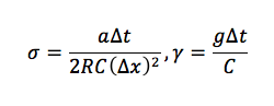
In order to remove the time differential, we apply the Crank-Nicholson method, which takes the equations at t = n and t = n+1, combines them, and brings common terms together to obtain:
This is an interesting equation. It removes the dependance of V on space(x), but not entirely. Instead of a differential, the voltage for any compartment (i) now depends on the voltage values of the compartments before and after it!
In order to remove the time differential, we apply the Crank-Nicholson method, which takes the equations at t = n and t = n+1, combines them, and brings common terms together to obtain:
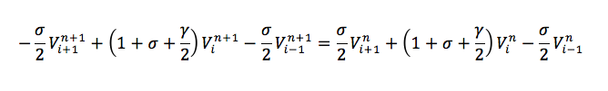
Where the superscript of V indicates time and the subscript indicates position, and
Now take a look at the equation above. all those coefficients can be thrown into constants to give a general equation as follows:
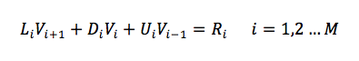
One point to be noted here - How did the three Vs in the RHS of the previous expression get reduced to a single R term in this one? Well, the entire RHS of the previous equation are values at time t=n. We know exactly what the system looks like at this point. So this expression will reduce to a single value. This is what R in the above equation denotes.
When represented in matrix form, this equation will form what is called a tri-diagonal matrix. Let's take a look at how that happens.
When represented in matrix form, this equation will form what is called a tri-diagonal matrix. Let's take a look at how that happens.
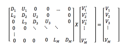
This is the matrix that we need to solve in order to get new voltage values (V') from old voltage values (V).
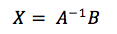
Now this matrix is in the form AX = B. We have A and B and need to solve for X. The way we do this is by inverting A and multiplying it to the left of both sides of the equation to get:
Now this matrix is in the form AX = B. We have A and B and need to solve for X. The way we do this is by inverting A and multiplying it to the left of both sides of the equation to get:
Getting the inverse matrix of A is a rather time consuming task. This is the main focus area while parallelizing this algorithm. Fast algorithms exist for general purpose inversion of matrices, but for this particular application, it is wasteful to use them directly. This is because, being a sparse matrix, such algorithms will spend a lot of processor time working on many elements which are 0s. Instead, we create a new form of representing this sparse matrix compactly and work on that matrix instead.
Note: The method above simply assumes that one compartment has only two neighbouring compartments. What about branches? Compartments can have any number of neighbouring compartments at the nodes of branches! Turns out this doesn't affect our calculations by all that much. The only change is that there will be some non-tridiagonal elements (elements that are not on the diagonal, lower diagonal or upper diagonal). We can ensure this using the Hines' method of node numbering. Once this is done, we can still solve for the matrix, keeping the off-diagonal elements in mind while performing Gaussian elimination.
So that was a pretty intensive post on the computational principles underlying the simultions in MOOSE. However, this puts us in a far better position to understand the actual code that carries out these functions in MOOSE. That is what the next post will be about.
 RSS Feed
