As I mentioned in my last post (quite a while back!), I will spend the next few posts going through the current implementation of the Hine's Solver in MOOSE. MOOSE has a folder called hsolve inside which there are a bunch of files for the implementation of the Hine's Solver.
The code for the Hines Solver is split into a couple of elements - the HSolve, HSolve Active and HSolve Passive classes.
The starting point to understanding this code is at hsolve.cpp. Here, a class called HSolve is defined. Objects of this class take over control when the Hines Solver is being used. As can be seen, this is a MOOSE class, with all the required elements - initCinfo, process and reinit functions etc.
Note how the process, reinit and setup functions of the HSolve class calls the respective functions in the HSolveActive class, which in turn calls the respective functions in the HSolvePassive class.
The HSolveActive class mainly deals with channel current calculations - the changes in current that happen between two compartments. The HSolvePassive class deals with the actual gauss jordan elimination procedure that provide the new voltages at each segment of the cell.
It also performs calculations for Calcium concentrations, which happen simultaneously with the current calculations.
When the target of the Hines Solver is set, the zombify function is called which disconnects the actual elements of the neuronal model from their clocks (so that they wont be doing any calculations anymore) and generates zombie versions of each element (which just pass processor control to the hines solver).
My main area of interest is the HSolvePassive Class where the forward elimination and backward substitution take place. So this is what we will look at here.
Since the Hines Matrix is a sparse matrix (There are a lot more 0s in the matrix than other numbers), it makes sense to represent the matrix in some other more compact form while doing calculations. This is the HS_ matrix. It reduces the large Hines matrix into a nx4 matrix with each compartment having just 4 values. Here is a small example to show how this HS_ matrix is generated.
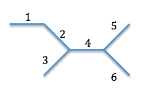
Consider the following compartmental model. The Hines indices of each compartment have been indicated:
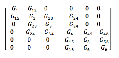
By the Hines method, this will result in the matrix shown below
Where the Ys are the admittances of that particular compartment and Zs are admittances of neighbouring compartments.
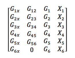
As you can see, this is a sparse matrix. To obtain a HS_ matrix from this, we pull out the relevant values from it and put it into another matrix. HS_ looks like:
As you can see, this is a sparse matrix. To obtain a HS_ matrix from this, we pull out the relevant values from it and put it into another matrix. HS_ looks like:
Where Y1x is the admittance at compartment 1 including external current influences, and X1 is the external current provided at compartment 1.
Admittance produced at junctions between two compartments are stored in a separate vector called HJ_. This is quite straightforward. Each junction admittance is specified one after the other in a long list of values. The way these junction currents are calculated is worth taking a look at.
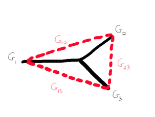
When just two compartments meet at a junction, the admittance between the two is straightforward to calculate. However, when more than two compartments meet at a junction, the junction needs to be broken down into a set of junctions each having just two compartments. For a junction with three compartments, this can be done as shown (The black lines are the actual compartments):
In such a case, the admittance at the junction is calculated using the equation Gij = Gi x Gj / Gsum . Gsum is the sum over all Gi.
Remember that the HJ_ vector stores only the values of admittances at all the junctions. There is no information on which junctions have which values! This mapping is done in two other vectors called junction_ and operandBase_.
This is a rough overview of the datastructures used in the Hines Solver. Note that this is true only for the current serial implementation. The next post will be on the actual forward elimination and back substitution algorithms that have been implemented.


 RSS Feed
