Blog Archives

Compiling CUDA code along with other C++ code

7/10/2014

This post will focus mainly on how to get CUDA and ordinary C++ code to play nicely together. This seemed like a pretty daunting task when I tried it first, but with a little help from the others here at the lab and online forums, I got it to work.
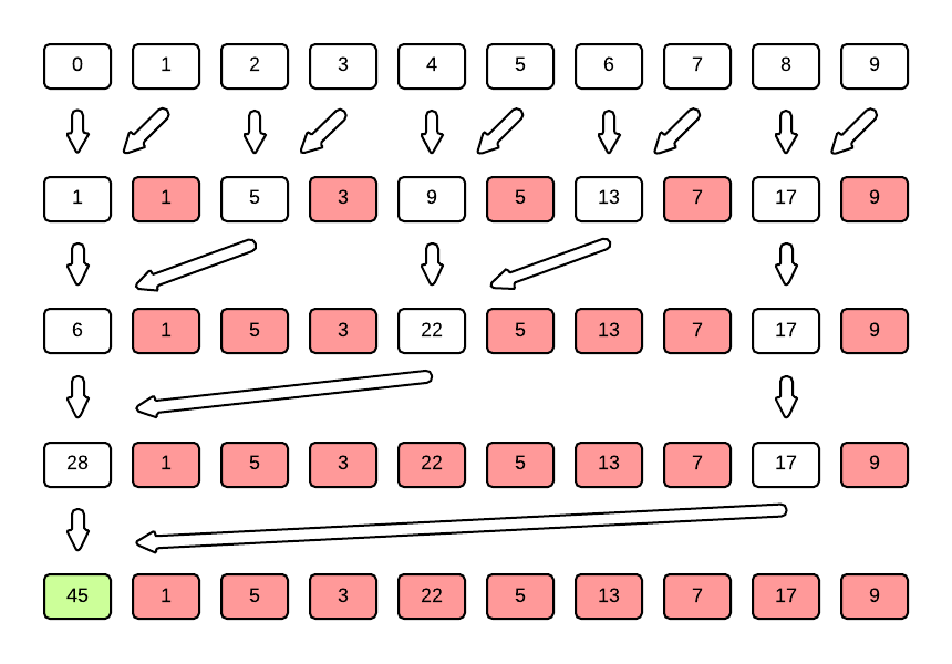
As a starting point, I used the code that was shown in the previous post - The summation from 1 to n. This code was put into a class called GpuInterface in GpuSolver.cu and it also had a GpuSolver.h header file. The files are shown below:
GpuSolver.h

#ifndef EXAMPLE6_H
#define EXAMPLE6_H
class GpuInterface
{
public:
int n[20];
int y;
int asize;

GpuInterface();
int calculateSum();
void setY(int);
};
#endif

GpuSolver.cu

#include <iostream>
#include <cuda.h>
#include "GpuSolver.h"

__global__

void findSumToN(int *n, int limit)
{
int tId = threadIdx.x;

for (int i=0; i<=(int)log2((double)limit); i++)
{
if (tId%(int)(pow(2.0,(double)(i+1))) == 0){
if (tId+(int)pow(2.0, (double)i) >= limit) break;
n[tId] += n[tId+(int)pow(2.0, (double)i)];
}
__syncthreads();
}
}

GpuInterface::GpuInterface()
{
y = 20;
asize = y*sizeof(int);
for (int i=0; i<y; i++)
n[i] = i;
}
int GpuInterface::calculateSum()
{
int *n_d;
cudaMalloc( (void**)&n_d, asize );

cudaMemcpy(n_d, n, asize, cudaMemcpyHostToDevice );

dim3 dimBlock( y, 1 );
dim3 dimGrid( 1, 1 );
findSumToN<<<dimGrid, dimBlock>>>(n_d, y);
cudaMemcpy(n, n_d, asize, cudaMemcpyDeviceToHost);
cudaFree (n_d);
return n[0];
}

void GpuInterface::setY(int newVal)
{
y = newVal;
asize = y*sizeof(int);
for (int i=0; i<y; i++)
n[i] = i;

}

And finally, I have a C++ file called main.cpp which just has a main function that creates a GpuSolver object and calls its functions, like so:

#include <iostream>
#include "GpuSolver.h"

int main()
{
GpuInterface obj;
obj.setY(16);
std::cout << obj.calculateSum();
return 0;
}

So the task now is to compile all of this into one executable. The key to understanding how we can do this is to understand how exactly the C++ compiler works. Professional computer science courses have a whole subject dedicated to Compilers, so I wont go into much detail. I'll just tell you that the compiler first converts the code (which is in a human readable format) into an intermediate code format. This is called assembly. The file created is called an object file. It contains essentially the same information as the source code file, but in a more machine-readable format. Separate object files are created for each source file in the project. Then, they are all linked together to form one single executable.
Typically, compilers automatically perform the assembly followed by the linking process. However, you can force it to stop after just the assembly, and then do the linking process later on. This is what we will have to do.

We run g++ on main.cpp with the -c flag that instructs g++ to stop compilation after the object files are generated. We also use the -I. flag to ask it to look for headers files within the current folder. The -o flag asks the compiler to call the output as whatever string follows the flag (in this case main.cpp.o). The full command looks like:

g++ -c -I. main.cpp -o main.cpp.o

We do a similar compilation on GpuSolver.cu with the following command

nvcc -c -I. -I/usr/local/cuda/include GpuSolver.cu -o GpuSolver.cu.o

Apart from the fact that g++ is replaced with nvcc (Nvidia CUDA Compiler) here, the only addition is the "-I/usr/local/cuda/include" flag. The path you see there contains some CUDA specific functionality that is required while compiling CUDA programs. So nvcc will need that library to compile the .cu file.

So now we have a bunch of files in our project directory:

main.cpp
GpuSolver.cu
GpuSolver.h
main.cpp.o
GpuSolver.cu.o

We now need to link the two .o files into one executable. We do this with the following command:

g++ -o exec GpuSolver.cu.o main.cpp.o -L/usr/local/cuda/lib -lcudart

Firstly, notice how we are just using the normal g++ call to perform the linking. g++ is clever enough to know that only the linking step is required and skips the assembly automatically. -o, like before, ensures that the output is named 'exec'. The files that need to be linked are specified next, followed by a -L and -l flag. The -L flag asks the compiler to look at the directory specified in the flag for additional files that may need to be linked. -l specifies the exact file that needs to be linked. Again, this is specific to CUDA.
When all of this has been done, you get a neat little executable that will calculate the sum from 1 to n!

I packed all of these commands into a makefile, which I've put down here

CUDA_INSTALL_PATH := /usr/local/cuda

CXX := g++
CC := gcc
LINK := g++ -fPIC
NVCC := nvcc

# Includes
INCLUDES = -I. -I$(CUDA_INSTALL_PATH)/include

# Common flags
COMMONFLAGS += $(INCLUDES)
NVCCFLAGS += $(COMMONFLAGS)
CXXFLAGS += $(COMMONFLAGS)
CFLAGS += $(COMMONFLAGS)

LIB_CUDA := -L$(CUDA_INSTALL_PATH)/lib -lcudart
OBJS = GpuSolver.cu.o main.cpp.o
TARGET = exec
LINKLINE = $(LINK) -o $(TARGET) $(OBJS) $(LIB_CUDA)

.SUFFIXES: .c .cpp .cu .o

%.c.o: %.c
$(CC) $(CFLAGS) -c $< -o $@

%.cu.o: %.cu
$(NVCC) $(NVCCFLAGS) -c $< -o $@

%.cpp.o: %.cpp
$(CXX) $(CXXFLAGS) -c $< -o $@

$(TARGET): $(OBJS) Makefile
$(LINKLINE)

For those of you wondering what just happened, welcome to the world of Linux makefiles :)
Makefiles are a way to script out the entire compilation and installation process for programs in linux. They have very weird syntax and there is no way I can explain all of it's details here. However, there are excellent tutorials on makefiles elsewhere on the internet, so I'd suggest doing some research.

The main point is that this makefile does almost exactly what I described above, with a bit of extra functionality for things like making sure the resulting executable can be further used in other programs, as opposed to needing to be run manually.

That's it for now! I'll leave the integration into MOOSE for next time.

2 Comments

Beginning GPU coding

7/10/2014

0 Comments

Trying to tackle the entirety of MOOSE directly wasn't working too well. So I am now working on parallelizing an example class. This can then be extended to HSolve where the GPU capabilities are actually required. This is a good exercising in understanding how to compile and run CUDA code alongside other CPU code, so I decided to document the entire process here.

The task I was given was simple - get a MOOSE class to calculate the sum of numbers from 1 upto some n, where n is defined by a member of that class. Then transfer the computation to the GPU while still maintaining an interface to MOOSE.

Setting up the MOOSE class

The example class I created is basically the same as the class I wrote about a few posts back. Do refer back to that post if you need a refresher on MOOSE classes.
The only change I made is in the process function. The class now calculates the sum of numbers from 1 upto y_ (one of its datamembers) and stores the result in x_ (another one of its datamembers). Heres the process function:

void Example::process( const Eref& e, ProcPtr p )
{
int count = 0;
for (int i=1; i<y_; i++)
{
count += i;
}
x_ = count;
}

The rest of the class is the same as before.
Now the aim is to shift this computation to the GPU. Ofcourse, being a GPU, we need to also develop a parallel algorithm to calculate this sum instead of just iterating through the array and summing the numbers. Let's create a new project where all the GPU coding can be done and later work on integrating that code into this class.

The Parallel Reduce Algorithm

This section will focus on programming the GPU to calculate the sum of numbers from 1 to n.
NOTE: You need to have a working installation of CUDA for this part. If you don't have one, a number of tutorials exist to guide you through the installation process. Complete that before you continue.

Every CUDA program has two parts - the main section and the kernel. The main section runs on the host (most often the CPU). Code written here is almost identical to ordinary C++ code. The kernel is where all the magic happens. This code is loaded into the device (the GPU) and will be run once by each computational unit within the GPU.
So the idea is that all the control is at the hands of the CPU, where you would write ordinary C++ code to control flow of instructions, while the actual data processing is done at the GPU, which will typically have small snippets of C++ code and a small amount of local memory but will run the same code multiple times in parallel. Together, they make a formidable number crunching machine!

Let's first take a look at the CPU code

int main()
{
int n[20] = {0};
int *n_d;
int y=20;

dim3 dimBlock( y, 1 );
dim3 dimGrid( 1, 1 );

const int asize = y*sizeof(int);

//1) Fill up the array with numbers from 1 to y
for (int i=0; i<y; i++)
n[i] = i;

//2) Allocate memory for the array on the GPU
cudaMalloc( (void**)&n_d, asize );

//3) Copy over the array from CPU to GPU
cudaMemcpy(n_d, n, asize, cudaMemcpyHostToDevice );

//4) Call the kernel
findSumToN<<<dimGrid, dimBlock>>>(n_d, y);

//5) Copy back the array from GPU to CPU
cudaMemcpy(n, n_d, asize, cudaMemcpyDeviceToHost);

//6) Free memory on the GPU
cudaFree (n_d);

std::cout << "\nSum: " << n[0]<< '\n';

return EXIT_SUCCESS;
}

The code is about as straightforward as you can imagine. Y is the limit until which we need to sum. In the unlikely case that the code isn't self explanatory, I have put down the steps here:

Generate the array having integers from 1 to y.
Allocate memory on the GPU to hold the array.
Copy the array from CPU to GPU.
Call the kernel y times.
Copy the array from GPU back to CPU.
Free memory on the GPU.

Let's take a look at some of the interesting aspects of this code.

The dimBlock and dimGrid definitions you see on top are a consequence of how computational units (CUs) are arranged in CUDA. The GPU contains a large number of computational units which are grouped together (in sets of 32, 64 etc) to form a block. Blocks are further grouped into a grid. CUDA also provides the helpful feature of identifying CUs within a block and blocks within a grid using 2 dimensional or even 3 dimensional coordinates. The actual arrangement in the GPU will be linear ofcourse, but this interface can be very helpful when dealing with applications in 2D space (like image processing) or 3D space(like point cloud analysis).
cudaMalloc is the GPU equivalent to malloc. It allocates the specified space on the GPU and points the specified pointer to the start address. The name of the pointer is n_d. The CUDA convention is to append _d to all pointers that are pointing to memory on the device.

NOTE: GPUs have a number of different levels of memory, each of which have specific tradeoffs between storage space and access speed. I haven't gone into those details here, but they are worth a read.

cudaMemcpy is again similar to memcpy, but does this between the CPU and GPU. Note that last parameter which determines which direction the memory is being copied.
findSumToN is a function call to a function that we haven't yet defined. This is the kernel, and I will come to this in a moment. Before that, take a look at the triple less-than and greater-than signs. Between them is the dimGrid and dimBlock that we defined earlier. This determines the number of kernels that are launched. In our case, dimBlock is (y, 1), so y CUs will be launched per block. Since dimGrid is (1,1), only one block will be launched. So that is y CUs in total, all launched linearly, within the same block. This is ofcourse not the best way to parallelize since a block might only be able to launch 32 threads (based on the GPU hardware) and theres a good chance y will be more than that. Nevertheless, this is enough for this project.
cudaFree, as you may imagine, just releases the memory pointed to by the pointer in its argument.

Before we look at the kernel, a brief introduction to the Parallel Reduce Algorithm will be helpful

What you see above is the reduce algorithm used with addition in its entirety!
The naive way of adding the numbers in an array is ofourse to take one element (usually the first) and keep adding each of the other elements to it until all the elements have been added. The resulting array will have the sum of numbers in it's first cell.
Here, the end result is the same, but the method is slightly different. We first take all even elements (every second element starting from the first) and add the element immediately after it. We then take every fourth element and add the element two spaces away. Then eighth, and so on until all the elements have been added.
The great thing about this approach is that it is far more parallelizable than the naive approach. To understand why, take a look at the first set of additions. Each addition takes 2 elements from the first array and puts the result into one element of the second array. None of those additions depend on values computed by any other operation. So all of them can be computed in parallel. The summation will have to pause after that first step though, to make sure all parallel units have finished computed the first level of summation before the next level of summation can be performed. This is called a synchronisation of threads.
So what will this look like in parallel code?

int tId = threadIdx.x;

if (tId%2 == 0)
n[tId] += n[tId+1];
__syncthreads();
if (tId%4 == 0)
n[tId] += n[tId+2];
__syncthreads();
if (tId%8 == 0)
n[tId] += n[tId+4];
__syncthreads();
if (tId%16 == 0)
n[tId] += n[tId+8];

Here, tId is the ID number of the thread being run. Remember how we started y computational units in that call to findSumToN? This is (a simplified version of) the code that they will run. Each of the y CUs are given a unique thread number which is used to identify them in the code.
So what exactly is happening here? All threads with odd tId will actually do nothing! This is a waste of CUs and should be avoided in production code. All threads with tId a factor of 2 will enter the first if branch. Here, they will compute the sum of the array element n[tId] and the element immediately after it. The __syncthreads() command instructs the GPU to force all CUs to wait until all other CUs have reached the same point. This will ensure that all the first level of calculations have been done, as mentioned before.
Then, all threads whose tIds are factors of 4 enter the second if branch where they add their element with the element two spaces away. This continues onward.
I have converted all of this into a generic function shown below:

__global__

void findSumToN(int *n, int limit)
{
int tId = threadIdx.x;

for (int i=0; i<=(int)log2((double)limit); i++)
{
if (tId%(int)(pow(2.0,(double)(i+1))) == 0){
if (tId+(int)pow(2.0, (double)i) >= limit) break;
n[tId] += n[tId+(int)pow(2.0, (double)i)];
}
__syncthreads();
}
}

Note that this is far from optimised code! There are way more calls to math functions than are required and many threads will be severely underused. It is, however, a fairly simple example to understand.

I originally planned to put down the entire process of making the GpuSolver class and integrating it into MOOSE over here, but this is becoming a very long post. So I'll stop here and finish it in the next post.

0 Comments

A quick revisit of the math behind HSolve

7/5/2014

0 Comments

A few days back I had the chance to talk to Niraj, the guy behind most of the HSolve related code in MOOSE. He ran through the entire math behind HSolve and I thought I should put that down here as it will help clear many of the doubts that you may be having. Let's start with the current equation for one compartment:

Now, out of these variables, some of them vary with time, while others stay constant. Let's take some time t=1. We will denote the time varying variables with a suffix 1. Then the equation for the ith compartment becomes:

Let us keep that equation aside for a moment and look at another bit of the derivation - The backward Euler method of approximation.
Understanding how this approximation is done is very simple with a diagram.

This is a (very) rough diagram to show how the approximation works. The blue line is a plot of some function F(n). Let's take two points on the X-axis, X0 and X1. We mark their locations on the plot as points C and A. Now, we take the slope of the function at A (given by the solid green line) and extend it back to the vertical line from X0. We then draw a line parallel to the just drawn line, starting from C and hitting the vertical line from X1. This is an approximation of the function at point X1 given it's value at X0 and it's slope at X1. This would predict the value of the function at X1 to be D, whereas the actual value is A.
This is how future values of the Voltages and Admittances are predicted in MOOSE.
So the equation used when performing Backward Euler Approximations is:

Now, we just replace dV/dt with the equation we got above. Remember that the C term which was on the Left Hand Side is brought down to the denominator of the RHS before substitution. That will give:

Taking all the V1 terms together, we get

We shift that last term to the LHS and take V1 out common to get

This can be simplified as follows by making the following substitutions

Where

So these coefficients you see are what actually goes into the Hines matrix. Aii are the diagonal terms, Aij are the off diagonal terms and Bi are the terms in the B matrix.
Hopefully, this will make the math behind HSolve a little more clear. It certainly helped me understand what was really going on.

0 Comments

Compiling CUDA code along with other C++ code

Beginning GPU coding

Setting up the MOOSE class

The Parallel Reduce Algorithm

A quick revisit of the math behind HSolve

Vivek Vidyasagaran

Archives

Categories